Frequently Asked Questions (FAQ)
What are Primitives?
The core philosophy behind our control concept is breaking down all electrochemical methods into their most basic primitives - primarily ramps and polarizations. These primitive operations serve as fundamental building blocks that you can combine and sequence to create a wide variety of electrochemical experiments, ranging from simple polarizations at different potentials to complex multi-step protocols.
This innovative approach allows researchers to design sophisticated electrochemical experiments by combining these fundamental components. You can assemble these primitives using the Custom Experiment Builder, which provides a visual programming interface that eliminates the need for traditional programming knowledge when designing experiments. For even greater flexibility in assembling primitives, you can use our Python or C++ APIs.
Zahner Lab experiments differ from primitives because they often combine multiple primitives or use preset parameters that aren’t displayed to the user. In contrast, the Custom Experiment Builder and APIs give you direct access to individual primitives. For example, the ramp primitive is available across software components as:
Zahner Lab
At the end of each Zahner Lab method, the blocks/primitives that make up the method are explained so that they can be assembled exactly as in the Zahner Lab with the Custom Experiment Builder.
Custom Experiment Builder
APIs
Python
zahner_link.meas.RampJob
Potentiostatic & Galvanostatic
The system supports both potentiostatic and galvanostatic operation modes, which you configure when switching on the potentiostat. The potentiostat can only switch between potentiostatic and galvanostatic when the potentiostat is switched on. The potentiostat must be switched off and on again to change the mode. Your choice of mode at switching on determines how all subsequent primitives are executed.
This means that Zahner Lab experiments and primitives differ because Zahner Lab experiments are listed separately for potentiostatic and galvanostatic operation modes with different names.
Important
A concrete example: if you are using galvanostatic mode and execute the Cyclic Voltammetry primitive (zahner_link.meas.CvJob, CV Block),
then although it is called CV, it is also executed in galvanostatic mode and the vertexes are currents in amperes.
The user must then switch off the potentiostat for a potentiostatic CV if they are using galvanostatic mode and then switch it back on again in potentiostatic mode for a potentiostatic CV.
Primitives vs Wave
There are two different ways of applying a signal to your cell, and the decision between them depends on how fast the signal changes.
Slow Signals: Ramp and Polarization
The ramp and polarization primitives are designed for slow processes. As a rule of thumb, this means individual steps or scans that last about ten seconds or longer and that are recorded at output data rates in the range of 50 Hz or below.
Before a primitive starts, the device has to configure it. This results in a short dead time between two consecutive primitives, during which the cell is neither controlled nor measured. For slow signals this dead time is negligible, because it is much shorter than the primitive itself. Any number of primitives can therefore be chained one after another without affecting the result. For the same reason, the polarization primitive enforces a minimum runtime of 0.5 seconds, which prevents you from using it in a range where the dead time would no longer be negligible. This value is an absolute lower limit and not a working point: the closer you get to it, the more the dead time influences your result. If you need shorter steps, use the wave primitive described below.
Both primitives support autoranging, and all of their parameters are entered directly in the block or job.
Fast Signals: Wave
For faster signals, such as pulse sequences, the dead time can no longer be neglected. Chaining short polarizations would leave gaps exactly in the time range you are interested in. These signals are therefore output with the wave primitive, which runs the complete waveform as a single primitive and thus without any gaps. This is also how the pulse methods of Zahner Lab work internally: DPV, NPV and SWV are all based on the wave primitive.
The wave accepts a list of current or voltage values, which are output one after another at a constant value rate. The output data rate at which the measured data is recorded is set independently of the value rate, so several measured points can be recorded per output value, as described in Sampling Rate vs Output Data Rate.
Because the wave is optimized for speed, it comes with two restrictions:
Autoranging is not available, as changing the current range takes far too long. You have to select a fixed current range that covers the expected current.
Current and voltage cannot be mixed within one wave, as switching the operating mode takes too long as well. Whether the values are output as voltages or as currents is determined by the mode in which the potentiostat was switched on.
Which Block or Job to Use
In the Custom Experiment Builder, the wave primitive is available as the Wave - Custom Waveform block. The block reads the values from a CSV file with one value per line, which makes it the right choice whenever you want to output a waveform that you have generated outside of Zahner Lab, for example a pulse sequence from a spreadsheet or a signal calculated with a script.
If your process is slow enough for the Ramp or Polarization block, use these blocks instead: they support autoranging and you do not have to prepare a file.
In the APIs, the wave is output with the zahner_link.meas.WaveFileJob.
The waveform is uploaded once as a resource, either from a binary array or from a file, and can then be output repeatedly.
The ArbitrarySignal.ipynb example notebook shows how a waveform is generated in Python,
uploaded as a resource and output with the zahner_link.meas.WaveFileJob.
Sampling Rate vs Output Data Rate
When working with primitives, you control the output data rate (ODR) - the frequency at which you receive measurement data points from the instrument. The ODR determines how often measurement results are delivered to your application.
Lower ODR settings allow the IM7 to perform more internal averaging between output points, which reduces noise in your measurements. Higher ODR settings provide more frequent data updates but with less internal averaging.
The instrument automatically determines its internal sampling rate based on your configured measurement channels. You can configure these channels via API or Zahner Lab, as described in the Channels chapter. This sampling rate is typically much higher than your specified ODR. The device continuously samples at this high internal rate, averages multiple samples together, and then delivers the averaged result at your chosen ODR. For optimal data quality, you should only measure the channels you actually need rather than all available channels, as enabling unnecessary channels decreases the internal sampling rate and reduces both averaging capability and overall data quality.
Example: During a slow OCV scan with a 10 Hz ODR, the device might sample internally at 100 kHz. In this case, every data point you receive represents the average of 10,000 internal measurements, delivered 10 times per second.
Autoranging
Most primitives support autoranging, which automatically adjusts the current measurement range based on the signal being measured. However, changing current ranges takes time - typically several tens of milliseconds, depending on your specific instrument.
Because of this delay, autoranging only works effectively with slower measurement processes. For fast electrochemical processes, autoranging can actually cause you to miss important data.
Example: Consider Cyclic Voltammetry (CV) with very fast scan rates. When an electrochemical reaction occurs and current begins flowing, the instrument detects this and switches to an appropriate current range. During the range-switching period, the instrument cannot measure current. Meanwhile, the potential scan continues, so by the time the range change is complete, the current peak may have already passed.
Important
If you know the expected current range for your experiment, it is recommended that you disable autoranging and select the appropriate range manually. This also applies to galvanostatic methods: even though you define the current of the primitive, the current range is a separate hardware setting that you must still configure manually to match your applied current once autoranging is disabled. This approach provides better data quality and prevents missing transient events.
Warm-up & DC Calibration
All Zahner instruments require at least 30 minutes of warm-up time before you begin taking measurements. This warm-up period is essential for the instrument to reach optimal precision and stability.
After the warm-up period, we recommend performing a DC calibration to ensure measurement accuracy. The IM7 performs this internal DC calibration automatically upon execution of the command, no external connections are required. The IM7 never performs automatic calibrations, these must always be triggered manually. This differs from Thales, where automatic calibrations were performed at various points, such as when selecting an EPC device.
Without proper calibration, measurement precision may be compromised. Additionally, performing DC calibration on a cold device will result in lower quality measurement data. Calibration takes approximately three to five minutes, depending on the number of add-on cards used.
EIS Waves & Duration
To optimize measurement time and data quality for each frequency point in EIS, two parameters are used: waves and duration.
waves sets the minimum number of sine wave cycles to measure.
duration sets the minimum time (in seconds) for the measurement.
There are separate settings for the settling period before measurement and for the actual measurement:
pre_waves and pre_duration: Control the settling period before the main measurement.
meas_waves and meas_duration: Control the main measurement period.
The instrument always measures at least meas_waves cycles. If the meas_duration has not been reached after those cycles, measurement continues until the time limit is met. At low frequencies, the number of measured waves will often be greater than the duration in seconds.
Examples:
1 Hz measurement frequency, meas_duration = 9, meas_waves = 3 ➡️ 9 waves are measured (since 3 waves would only take 3 seconds)
1 Hz measurement frequency, meas_duration = 0, meas_waves = 3 ➡️ 3 waves are measured
Stop Conditions
Stop conditions allow you to automatically terminate a primitive before its normal completion based on specific criteria you define. This feature adds intelligent control to your experimental protocols, making them more responsive to real-time conditions.
How Stop Conditions Work
Stop conditions are evaluated at each data point according to your specified output data rate (ODR). This means your ODR setting directly affects how quickly a stop condition can be detected and acted upon. For time-sensitive stop conditions, make sure to set an appropriately fast ODR.
Practical Applications
Stop conditions enable sophisticated experimental designs that adapt to your sample’s behavior:
Constant current charging: Use a
zahner_link.meas.PogaJobwith a voltage-based stop condition to automatically end charging when your target voltage is reachedOpen circuit voltage monitoring: Set up an OCV scan that stops automatically once the voltage stabilizes within your specified tolerance
Safety limits: Prevent damage by stopping experiments when current, voltage, or other parameters exceed safe ranges
Available Stop Conditions
Complete documentation for stop conditions is available for each platform:
Impedance and Channel Statistics
The IM7 provides comprehensive statistics for impedance measurement results. Each channel involved in impedance measurements includes total harmonic distortion (THD) and drift metrics.
For impedances and phases calculated using two channels, the system provides standard deviation and drift statistics for each.
THD
Total Harmonic Distortion (THD) quantifies signal distortion caused by harmonics. Using standard signal processing calculations, THD is defined as the ratio of the sum of all harmonic component powers to the fundamental frequency power.
Standard Deviation
Standard deviation measures the variability or dispersion of impedance measurements at a specific frequency point.
This calculation follows standard scientific practices. However, standard deviation can only be determined when multiple waves per impedance point are measured.
Drift - Channels
Calculated as a percentage of the ADC full scale, normalized as drift per period of the applied sine wave. (100% = 1.0 = Full Scale per Period)
Drift - Impedance & Phases
Drift represents the total amount of drift that occurred during the measurement of a single impedance point at a specific frequency, excluding the prewave period.
Values are expressed in Ohms or Degrees of drift per measurement of a single impedance point.
Stationarity and Linearity in EIS
Electrochemical Impedance Spectroscopy (EIS) relies on two fundamental assumptions about the system under test: stationarity and linearity. Violating either of these conditions leads to unreliable or meaningless impedance data.
Why Stationarity and Linearity Matter
Stationarity means that the electrochemical system must not change during the measurement. Since EIS sweeps through many frequencies one by one, the full measurement can take a significant amount of time, particularly at low frequencies. If the system drifts, corrodes, or otherwise evolves during this period, the impedance values measured at different frequencies no longer describe the same system state. This makes the resulting spectrum internally inconsistent and difficult to interpret.
Linearity means that the system must respond linearly to the applied excitation signal. EIS applies a small sinusoidal voltage or current perturbation at each frequency and measures the response. If the perturbation amplitude is too large, the system enters a non-linear regime. In a non-linear regime, the response is no longer a pure sine wave at the excitation frequency. Instead, additional frequency components, so-called harmonics, appear in the response signal. These harmonics distort the impedance measurement and make the results unreliable.
Verifying Linearity from Waveform Data
The IM7 provides the raw waveform data (voltage and current sine waves) for each frequency point during an EIS measurement. Zahner Lab provides two dedicated dashboard displays to help you verify linearity in real time during the measurement:
The Wave Display shows the measured voltage and current waveforms (solid lines) together with their extracted fundamental waves (dashed lines).
The FFT Display shows the frequency-domain decomposition of the waveforms, revealing any harmonic components.
These dashboards are powerful tools that allow you to evaluate signal quality live while the measurement is running, so you can immediately detect problems and adjust the amplitude if necessary.
The following figure shows an example of a distorted galvanostatic EIS measurement as displayed in the Zahner Lab dashboards:
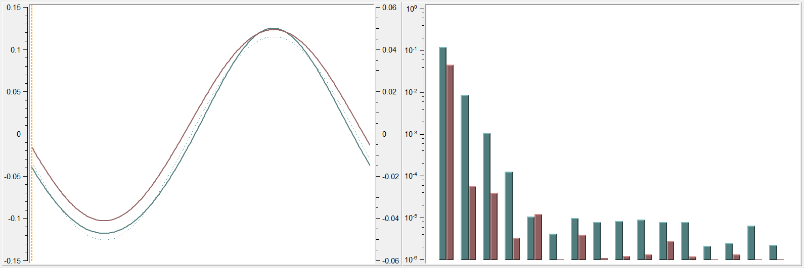
In the left plot (Wave Display), the voltage waveform (blue, solid line) deviates significantly from its extracted fundamental wave (blue, dashed line). Since this is a galvanostatic measurement, the current is the excitation signal and remains a clean sine wave, while the voltage is the response signal. The visible distortion of the voltage waveform indicates that the system has been driven into a non-linear regime by the applied current amplitude.
In the right plot (FFT Display), this non-linearity becomes clearly quantifiable. The blue bars representing the voltage signal show significant energy in the 2nd, 3rd, and higher harmonics, with the harmonic levels being only a factor of 10 lower than those of the fundamental frequency. In contrast, the red bars representing the current excitation signal show much smaller harmonics. This asymmetry between the excitation and response harmonics is characteristic of a non-linear system response.
The THD (Total Harmonic Distortion) value, described in the Impedance and Channel Statistics section above, quantifies this distortion as a single number.
Choosing the Right Amplitude
To ensure linearity, you should select an excitation amplitude that is small enough to keep the system in the linear regime. As a general guideline, the voltage amplitude is often kept in the range of 5 to 20 mV for potentiostatic EIS. However, the appropriate amplitude depends on the specific electrochemical system.
The Wave Display and FFT Display in the Zahner Lab dashboards are specifically designed to guide you through this process. By monitoring these displays during a measurement, you can iteratively adjust the amplitude until the system operates in the linear range.
The following figure shows the dashboards for a measurement where the amplitude has been correctly chosen:

In the left plot, the measured voltage and current waveforms closely overlap with their respective fundamental waves. There is no visible distortion, confirming that both signals are clean sine waves.
In the right plot, the FFT shows that the harmonic components are several orders of magnitude below the fundamental frequency for both voltage and current. This confirms that the system is operating well within the linear range.
When the dashboards show this kind of clean signal, you can be confident that the chosen amplitude is appropriate and the impedance data is reliable. If you observe significant harmonic content or visible distortion in the waveforms, reduce the excitation amplitude and repeat the measurement until the dashboards confirm linearity.
Extracting and Analyzing Waveform Data with Python
The EisWaves.ipynb example notebook demonstrates how to:
Access the raw voltage and current waveform data for each frequency point after an EIS measurement
Visualize the waveforms using matplotlib
Assess the signal quality to check for non-linear distortion or measurement artifacts
This is particularly useful for post-measurement verification that the system was operating in the linear range during the entire EIS sweep.
It is very important to note that impedance cannot be calculated directly from the waves. To do this, the complex calibration algorithms for the entire signal chain would have to be applied, which the measuring device performs internally to calculate the impedance. The wave represents the modulation of the converters and is only used to estimate the signal shape, whether it is distorted or noisy, or whether other artifacts are visible.